Brief overview

A survival analysis is conducted on the OpenPowerlifting.org dataset. Individual powerlifters and the length of time that they’ve been active (in terms of time from first to last meet and number of meets attended) are treated as survival objects. Survival curves are fitted and covariates are examined for effects.

This project was completed in part as a semester project for a Reliability Data Analysis course at the University of South Florida. This project was completed with the help of my project partner, Kheycie Romero .

Introduction

If you practice a sport long enough, it is inevitable that you will see new people come and go. A common observation in Brazilian Jiu Jitsu is that of the “blue belt blues” - people who get their blue belt (the first major belt promotion) and then stop showing up to classes not long afterwards.

With any sport, the risk of injury and the pressures that come with age and its responsibilities will, over time, cause people to drop out of the sport. OpenPowerlifting.org provides a dataset that allows us to examine this phenomenom in surprising depth for the sport of Powerlifting.

Data Exploration & Feature Engineering

Our starting dataset consists of 822,869 observations. Each row represents the performance of a single powerlifter in a single event at a single powerlifting meet. Each row gives a powerlifter name, sex, age, age class, bodyweight, weight class, country of origin, and the following information about the event: an abbreviation giving event type, the event division, the event country, the event federation, the date of the event, the state of the event, the meet name, the Wilks, McCulloch, and Glossbrenner scores for their performances, and their performances in various lifts.

A sample row can be seen below:

1
2
3
4
5
6

> pldat[6,]
             Name Sex Event Equipment Age    Division BodyweightKg WeightClassKg Squat1Kg Squat2Kg Squat3Kg Squat4Kg Best3SquatKg Bench1Kg Bench2Kg Bench3Kg Bench4Kg Best3BenchKg Deadlift1Kg Deadlift2Kg
6 Courtney Norris   F   SBD     Wraps  28 Open Senior        62.41          67.5   145.15   158.76    170.1   -183.7        170.1    77.11   -86.18   -86.18       NA        77.11      129.27      145.15

  Deadlift3Kg Deadlift4Kg Best3DeadliftKg TotalKg Place Wilks McCulloch Tested AgeClass Country Glossbrenner Federation       Date MeetCountry MeetState                                            MeetName
6     -161.03          NA          145.15  392.36     1 424.4     424.4     No    24-34               374.79  365Strong 2016-10-29         USA        NC Junior & Senior National Powerlifting Championships

In order to examine the competitive lifetime of powerlifters, we have to conduct a number of transformations on the data. First and foremost, we want a new dataset that consists of information about individual powerlifters. That is, we want each row in this dataset to represent a single powerlifter. This process is carried out below.

Note: the code for some of the original work on this project was lost. As a result, the code for engineering the new dataset is replicated below on a small subsample of the data in order to save time.

 1
 2
 3
 4
 5
 6
 7
 8
 9
10
11
12

> small_pld <- pldat[sample(nrow(pldat), 5000),]
> small_lifters <- unique(small_pld$Name)
> liftindices <- lapply(small_lifters, FUN=function(x) which(small_pld$Name == x))
> liftdates <- lapply(liftindices, FUN=function(x) lapply(x, FUN=function(x) as.Date(small_pld[x,]$Date)))
> small_liftdf <- as.data.frame(small_lifters)
> small_liftdf$Dates <- liftdates
> first_meet <- lapply(liftdates, FUN=function(x) min(unlist(x)))
> last_meet <- lapply(liftdates, FUN=function(x) max(unlist(x)))
> small_liftdf$First_Meet <- first_meet
> small_liftdf$Last_Meet <- last_meet
> small_liftdf$First_Meet <- as.Date(unlist(small_liftdf$First_Meet), origin="1970-01-01")
> small_liftdf$Last_Meet <- as.Date(unlist(small_liftdf$Last_Meet), origin="1970-01-01")

A few notes about the above: working with Dates in R is not as easy as one would like, particularly when having to work with lists of dates. Unlisting dates automatically converts them to a numeric format that uses 1970-01-01 as the origin. However, to use “as.Date()” on a date, you must specify the origin, and if you specify the origin incorrectly (i.e. if you do not know the default date), the dates will be incorrect. You’ll also note that everything was done using the vectorized lapply function - this turned out to be simpler than trying to use apply over each row of the dataframe.

The dataframe created above is sufficient to generate survival objects. Our final step was to collect covariates using similar methods as above.

After collecting covariates, we omitted all rows that had NA’s. This is not generally a great practice and we could work around rows with NA’s, but we have so much data here that it shouldn’t be a significant issue.

We generated age classes (so that we could treat age as a categorical rather than continuous variable - a sacrifice that proves useful when creating survival plots):

1
2
3
4
5

> ldf$AgeClassifier <- "<20"
> ldf[ldf$StartAge >= 20 & ldf$StartAge <= 29,]$AgeClassifier <- "20-29"
> ldf[ldf$StartAge >= 30 & ldf$StartAge <= 39,]$AgeClassifier <- "30-39"
> ldf[ldf$StartAge >= 40 & ldf$StartAge <= 49,]$AgeClassifier <- "40-49"
> ldf[ldf$StartAge >= 50,]$AgeClassifier <- "50+"

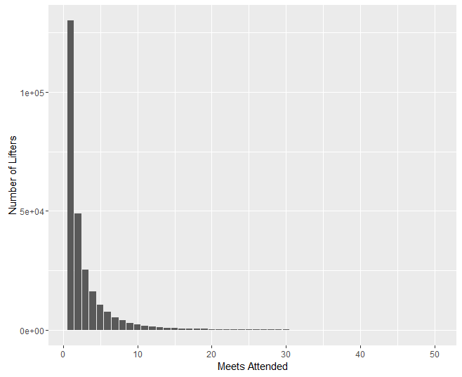
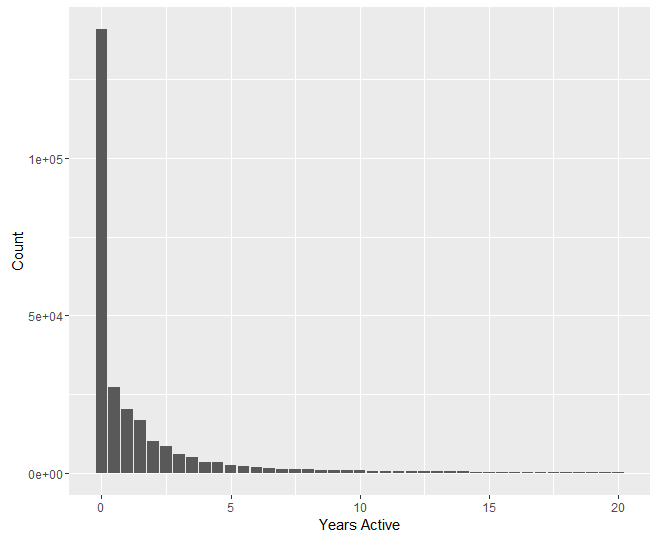
We now have two potential measures for competitive lifetime: number of meets attended, and time from first meet to last meet. Our analyses will be conducted using both of these measures. We first plot survival counts in terms of both measures. These plots were created with R’s ggplot library.

Preliminary Analyses

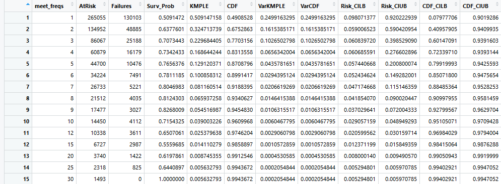
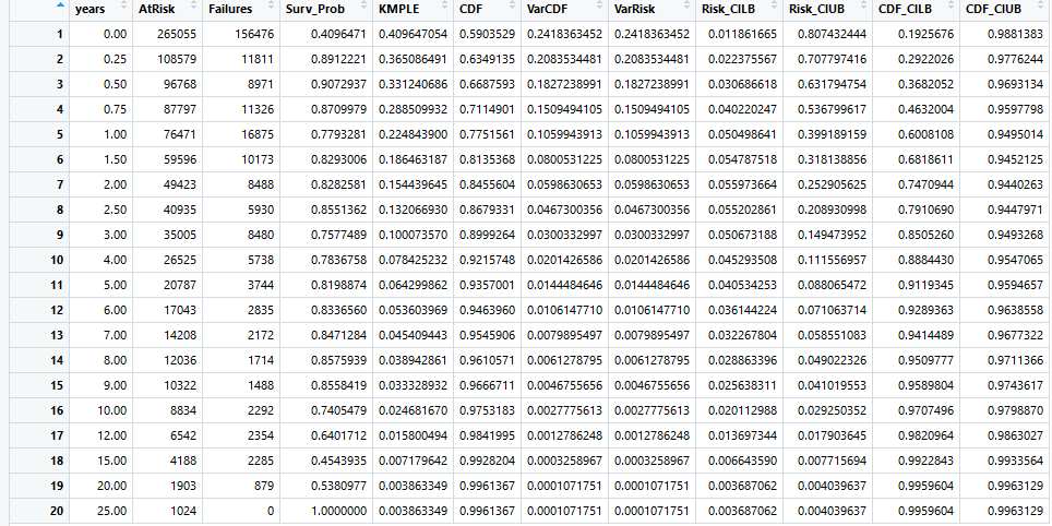
We first carry out a non-parametric analysis of our survival data by creating a Kaplan-Meier Product Limit Estimator (KMPLE) table and curve for both forms of lifetime. These can be seen below. Note that for the Years KMPLE plot, a slight modification was made that is not visible presently in the tables: anyone who attended only one meet would appear as active for 0.00 years, which was adjusted to 0.083 years (1 month) when creating survival objects. The surv package in R does not allow survival times of 0.00.

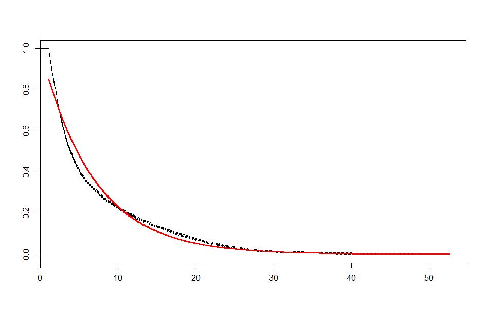
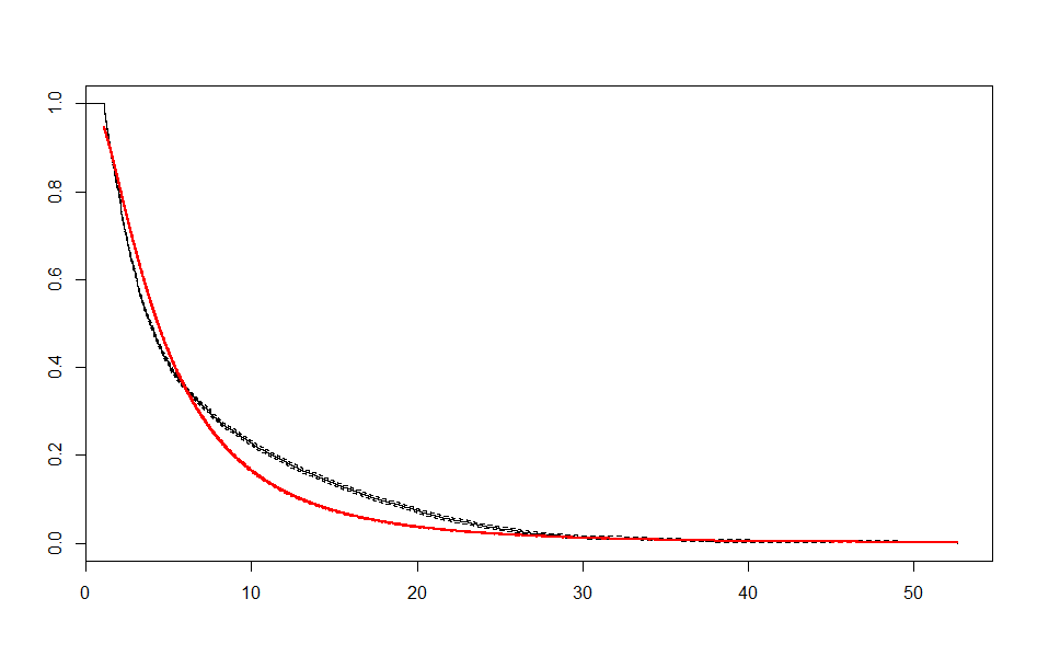
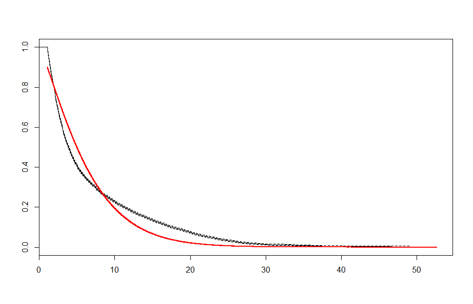
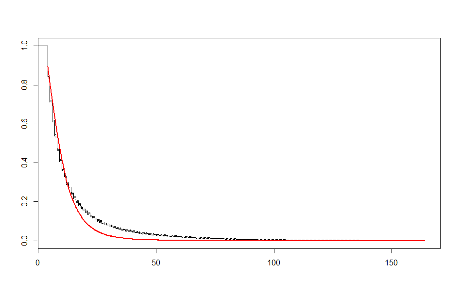
Finally, we do a preliminary fit of some common parametric curves to examine if any of these fit the data well. These can be seen below:

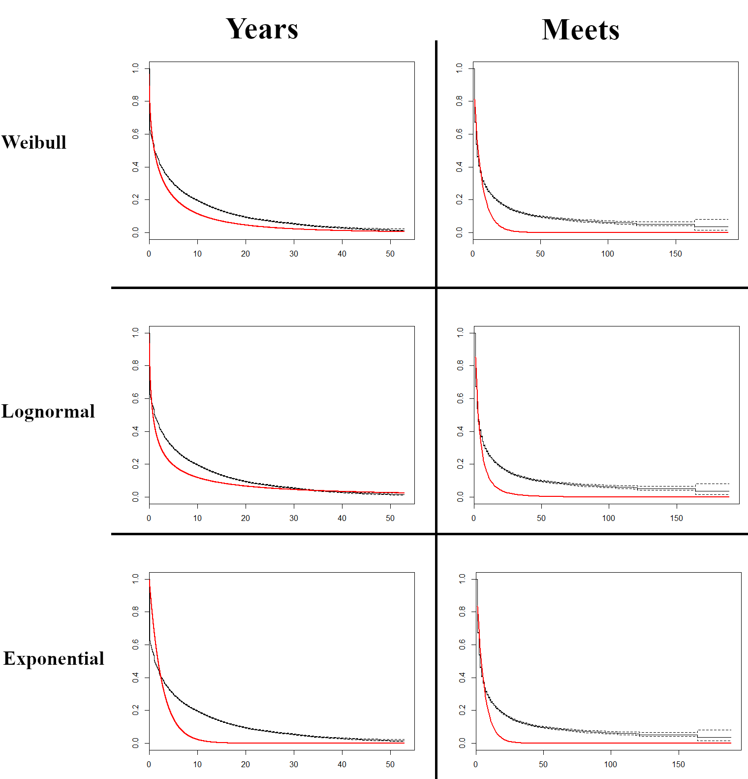
Each of the curves show significant regions of misfit. Given that none of the common parametric curves are a good fit for the data alone, we next want to examine covariates, and may thereafter conduct a semi-parametric analysis.

Examining Covariates

We next want to identify and examine our covariates. The most obvious covariates are the biological ones: gender, age, and bodyweight. Feature engineering may present new covariates, such as the performance of the powerlifter at their first meet, the frequency of meet attendance, change in biological variables (e.g. moving to a new bodyweight or age class), et cetera.

We examined some of the most obvious covariates:

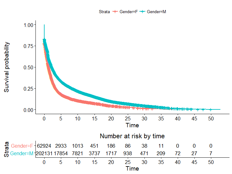
Here we see a well defined difference in survival among the genders. Women have a much steeper drop-off, tending to remain competitive for much shorter periods of time. This trend is especially well defined after that initial “drop off” period.

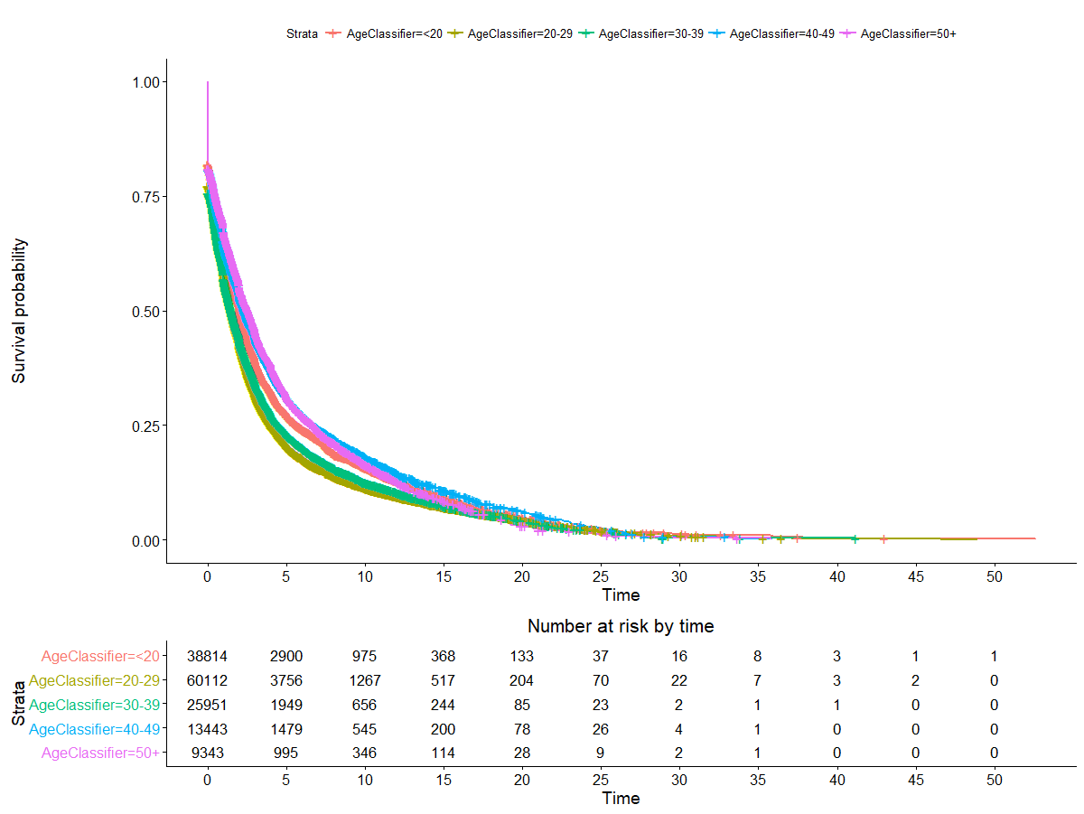
The relationship here is less clear. There does appear to be a difference in survival by age class, but it’s not super well defined and seems more or less to fit with the expectation that older lifters are less likely to stay on the competitive scene. The only exception here is people who started under 20. This may be worth examining later.

Survival curves and plots were fitted using the survival and survminer libraries in R.

Fitting a Semi-Parametric Model

Now that we have a number of covariates to explore, we attempt to fit a semi-parametric model. For this, we use the Cox Proportional Hazards model.

The Cox-PH model fits a hazard function to survival data using multiple linear regression. The model essentially multiplies a baseline hazard (the hazard when all variables are equal to 0) by an exponential function containing a linear combination of covariates.

$ h(t) = h_{0}(t) \times exp(b_{1}x_{1} + ... + b_{k}x_{k}) $

Because of the model’s form, the covariates must meet a set of constraints, namely:

1. Hazard functions for different levels of each covariate must be proportional over time - they should not overlap
2. Any censoring should be non-informative
3. The relationship between the log hazard and each covariate should be linear.

We will check these assumptions in time. For now, we fit a model:

 1
 2
 3
 4
 5
 6
 7
 8
 9
10
11
12
13
14
15
16
17
18
19
20
21
22
23
24
25
26
27

> cphmod <- coxph(Surv(TA_Years,Active)~Gender+StartAge+StartWeight+StartWilks, data=ldf)
> summary(cphmod)
Call:
coxph(formula = Surv(TA_Years, Active) ~ Gender + StartAge + 
    StartWeight + StartWilks, data = ldf)

  n= 147663, number of events= 76390 

                  coef  exp(coef)   se(coef)      z Pr(>|z|)    
GenderM     -3.850e-01  6.804e-01  9.036e-03 -42.61   <2e-16 ***
StartAge    -6.049e-03  9.940e-01  3.234e-04 -18.70   <2e-16 ***
StartWeight  3.810e-03  1.004e+00  1.843e-04  20.68   <2e-16 ***
StartWilks  -8.465e-04  9.992e-01  2.788e-05 -30.36   <2e-16 ***
---
Signif. codes:  0 ‘***’ 0.001 ‘**’ 0.01 ‘*’ 0.05 ‘.’ 0.1 ‘ ’ 1

            exp(coef) exp(-coef) lower .95 upper .95
GenderM        0.6804     1.4696    0.6685    0.6926
StartAge       0.9940     1.0061    0.9933    0.9946
StartWeight    1.0038     0.9962    1.0035    1.0042
StartWilks     0.9992     1.0008    0.9991    0.9992

Concordance= 0.554  (se = 0.001 )
Rsquare= 0.019   (max possible= 1 )
Likelihood ratio test= 2847  on 4 df,   p=0
Wald test            = 2903  on 4 df,   p=0
Score (logrank) test = 2917  on 4 df,   p=0

The results aren’t super encouraging. While all of our variables appear to be significant, they don’t seem to have a terribly noticeable effect on the fit. The Rsquare for a Cox-PH model is a pseudo-R-squared that measures the improvement in likelihood of the fitted model over a model with no covariates (Thanks to EdM for this interpretation: https://stats.stackexchange.com/questions/145238/coxph-r-squared-interpretation-in-r ). Most of this additional fit comes from the gender variable - a Cox-PH model utilizing just that variable has an Rsquare of 0.01.

A further examination of the Schoenfeld residuals reveals additional issues. The cox.zph function in the survival package tests the proportional hazards assumption by measuring the relationship between scaled Schoenfeld residuals and time. Covariates showing significance in the test fail to meet the requirements of the covariates of a Cox-PH model. We test below:

1
2
3
4
5
6
7

> cox.zph(cphmod)
                rho  chisq        p
GenderM     -0.0371 106.51 0.00e+00
StartAge    -0.0184  24.46 7.61e-07
StartWeight  0.0311  66.31 3.33e-16
StartWilks   0.0123   8.62 3.32e-03
GLOBAL           NA 145.58 0.00e+00

The issues with these covariates could be resolved, but it seems likely to not be worth it in the long run. The results are even worse with survival objects based on meet counts instead of length of time active. We move on to other methods.

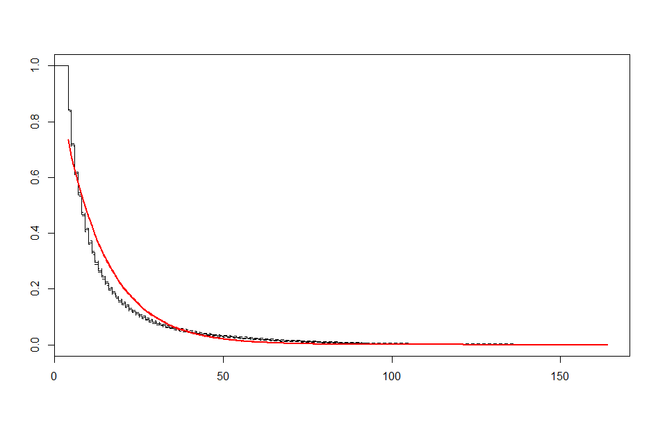
Fitting Modified Parametric Survival Curves

We initially attempted to fit parametric survival curves without covariates and without splitting the data into regions. We’ve since noted that there appear to be two separate “regions” of the data - the “early” region where most competitive lifters drop out, and then a more stable region where dropoff has slowed considerably. We’ve also noted that some covariates appear to have a noticeable effect on the survival curve.

We now turn to fitting parametric curves for separate covariates and for separate regions of the survival curve. First, we fit the parametric curves for separate regions.

 1
 2
 3
 4
 5
 6
 7
 8
 9
10
11
12
13
14
15
16
17
18
19

year_fit_parametrics <- function(data1, data2){
	dists <- c("exponential", "lognormal", "weibull")
	year_fits1 <- lapply(dists, function(x) flexsurvreg(Surv(Years_Mod, Active)~1, dist=x, data=data1))
	year_fits2 <- lapply(dists, function(x) flexsurvreg(Surv(Years_Mod, Active)~1, dist=x, data=data2))
	lapply(year_fits1, function(x) plot(x))
	lapply(year_fits2, function(x) plot(x))
	return(list(year_fits1, year_fits2))
}
> yearfits <- year_fit_parametrics(ldf1, ldfm1)


meet_fit_parametrics <- function(data1, data2){
	dists <- c("exponential", "lognormal", "weibull")
	meet_fits1 <- lapply(dists, function(x) flexsurvreg(Surv(MeetCount, Active)~1, dist=x, data=data1))
	meet_fits2 <- lapply(dists, function(x) flexsurvreg(Surv(MeetCount, Active)~1, dist=x, data=data2))
	lapply(meet_fits1, function(x) plot(x))
	lapply(meet_fits2, function(x) plot(x))
	return(list(meet_fits1, meet_fits2))
}

We end up with a set of plots that looks like this:

	Before 1 Year	After 1 Year
Exponential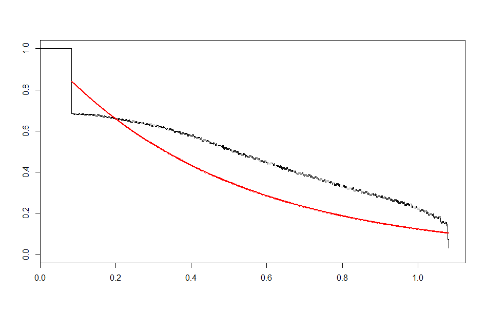
Lognormal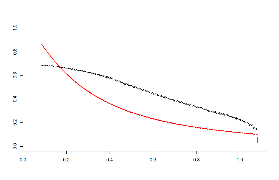
Weibull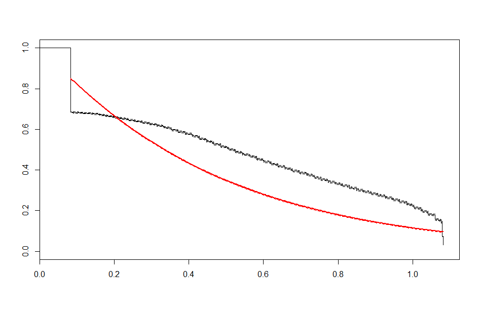

	Before 3 meets	After 3 meets
Exponential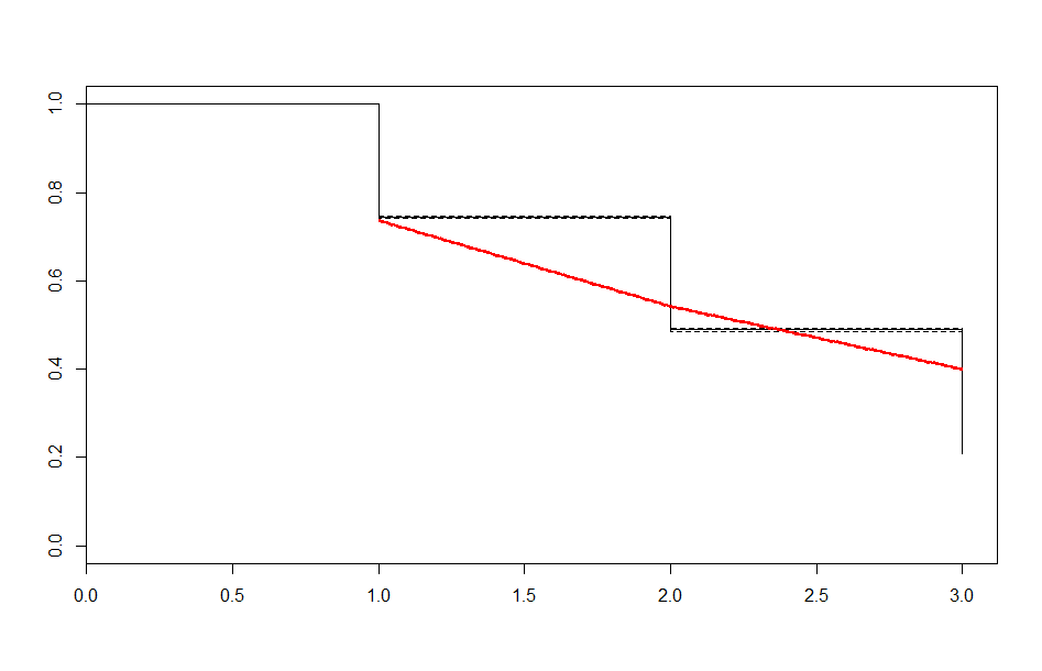
Lognormal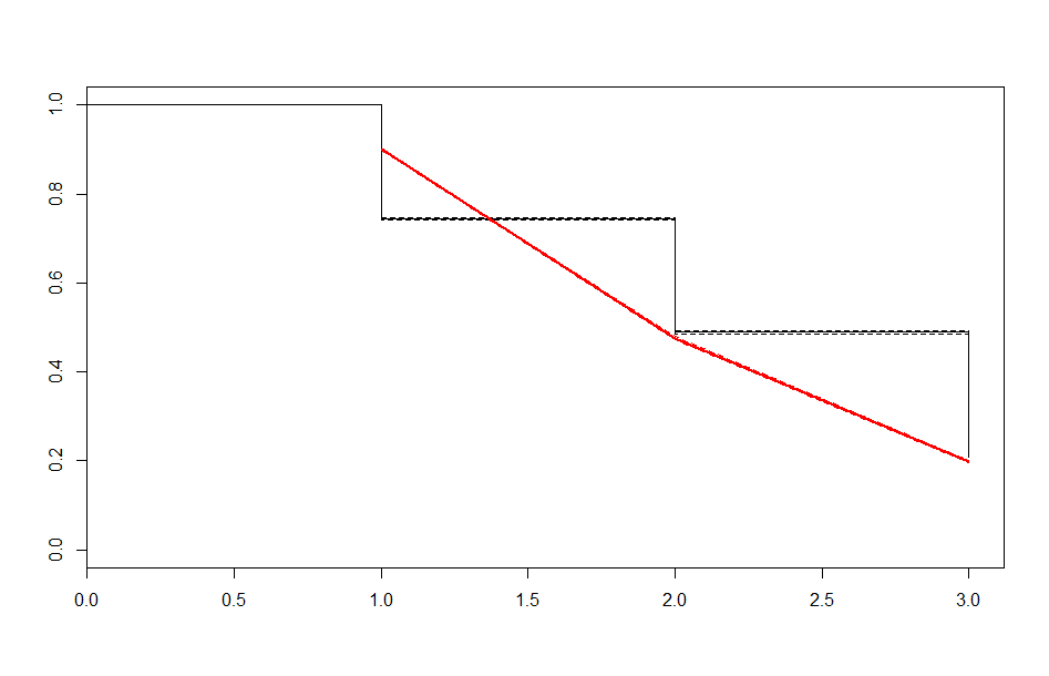
Weibull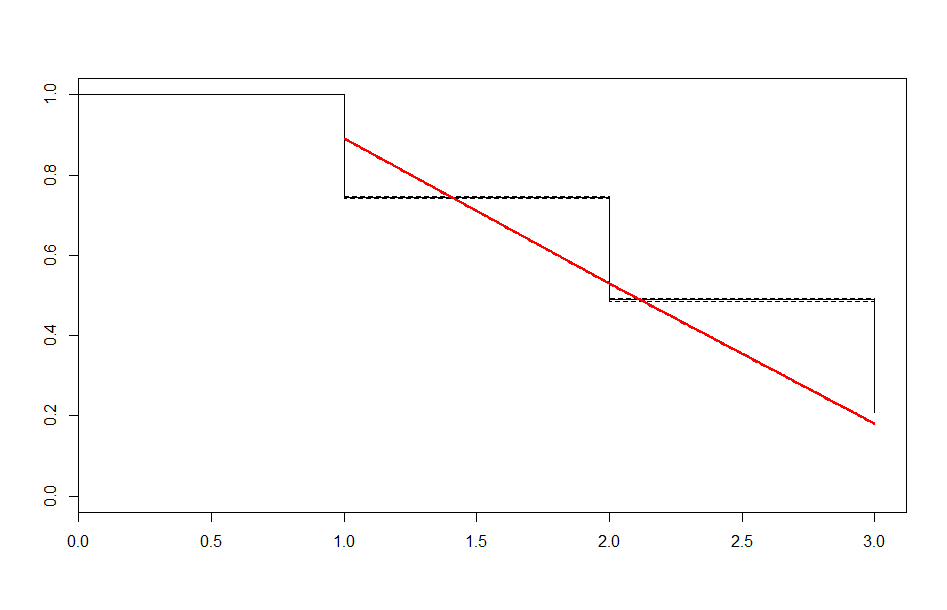

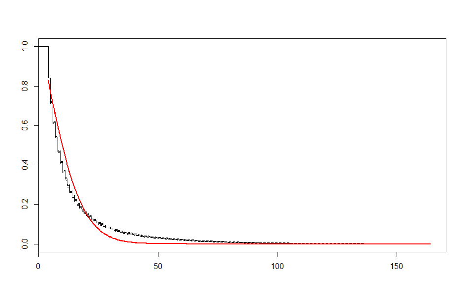These look better than the parametric plots we produced at the beginning. The cutoff was picked more or less by eyeballing it - we could likely do better than this. The fits definitely aren’t perfect, but they are suggestive - after some cutoff, the exponential distribution appears to be the best fit, which implies a constant hazard rate after some threshold.

Conclusions and Next Steps

We haven’t arrived at a final model yet. We have, however, arrived at a few important conclusions:

1. The most obvious covariates available to us are not as strongly predictive as we might think. Starting weight, starting age, and starting stats don’t appear to be extremely predictive of long term hazard, although gender does appear to play a big role.

2. A model for competitive lifetime seems likely to include a threshold of sorts - at some time point or number of meets, the hazard rate stops being determined by one distribution and begins being determined by another.

3. We have some evidence that the exponential distribution is more explanatory after some threshold cutoff, implying a constant hazard rate after that point. This falls in line with intuition - we’d expect a lot of people to try out the sport and quit not long after, leading to a lot of drop-off early on that levels off later.

Going forward, more work could be carried out in:

1. Engineering more covariates, whether by collecting data from additional sources or examining the present dataset for more features. We spent relatively little time on feature engineering at the beginning. It is likely to be worthwhile to go back to that soon.

2. Fitting parametric models that account for covariates.

3. Getting a better idea of where a threshold might lie for switching between parametric models, if we decide to stick with a parametric model.

4. Examining other semi- and non-parametric models that will allow us to explicitly include covariates in our model.