Just a quick experiment I was curious about! A few friends and I are starting up a new D&D campaign, and a player asked me how I prefer stats for characters to be determined. I’ve always preferred point buying, but I enjoy the randomness of rolling stats. I ran some simulations to get an idea of what kind of stat distributions different rolling methods give!

First, we define our functions for generating stats. The first function simply rolls X number of dice and keeps either the 3 biggest or 3 smallest, based on a user-specified option. We can use this to generate a set of six stats by calling the function 6 times - which is what the generate_stat_set() function does.

The next function is a bit more interesting: we roll 3 sets of 3d6 (which we can use our previous function for), then we use the 3 numbers generated to generate 3 more numbers that are “inverse” to what we got. What we set as the upper bounds for generating the inverse set will determine how powerful of characters are generated.

We also test a stat-set-generating function that performs a “best of …” roll - it generates two or more stat sets and keeps the “best” one. How we pick the “best” set matters a lot. In this case, we simply keep the set with the highest sum.

More methods will be added as I think of them!

 1
 2
 3
 4
 5
 6
 7
 8
 9
10
11
12
13
14
15
16
17
18
19
20
21
22
23
24
25
26
27
28
29

generate_stat <- function(numToRoll=3, MaxOrMin=TRUE){
	dice_face <- c(1, 2, 3, 4, 5, 6)
	draws <- sample(dice_face, numToRoll, replace=TRUE)
	keep <- draws[order(draws, decreasing=MaxOrMin)[1:3]]
	stat <- sum(keep)
	return(stat)
}

generate_stat_set <- function(numToRoll=3, MaxOrMin=TRUE){
	stat_set <- replicate(6, generate_stat(numToRoll, MaxOrMin))
	return(stat_set)
}

generate_inv_stat_set <- function(ub = c(24, 22, 20)){
	rolls <- replicate(3,generate_stat(numToRoll=3))
	rolls <- rolls[order(rolls, decreasing=TRUE)[1:3]]
	inv1 <- ub[1] - rolls[1]
	inv2 <- ub[2] - rolls[2]
	inv3 <- ub[3] - rolls[3]
	return(c(rolls[1], rolls[2], rolls[3], inv1, inv2, inv3))
}

generate_best_of_set <- function(bo = 2, numToRoll=3){
	sets <- replicate(bo, generate_stat_set(numToRoll, TRUE))
	sums <- lapply(1:bo, function(x) sum(sets[,x]))
	keep <- order(unlist(sums), decreasing=TRUE)[1]
	keepset <- sets[,keep]  
	return(keepset)
}

Next, we test our functions. We will do this by simply running the functions many times over and generating dataframes from the results. We’re going to examine the distribution of the sum and the median of the stat sets for a start.

 1
 2
 3
 4
 5
 6
 7
 8
 9
10
11
12
13
14
15
16
17
18
19
20
21
22
23
24
25
26
27

# 3 rolls, pick max 
> stat_sets_3rm <- replicate(1000, generate_stat_set(3, TRUE))
> stat_sets_3rm <- data.frame(t(stat_sets_3rm))
# 4 rolls, pick max
> stat_sets_4rm <- replicate(1000, generate_stat_set(4, TRUE))
> stat_sets_4rm <- data.frame(t(stat_sets_4rm))
# 4 rolls, pick min
> stat_set_4rmi <- replicate(1000, generate_stat_set(numToRoll=4, FALSE))
> stat_set_4rmi <- data.frame(t(stat_set_4rmi))
# Inverse stat set, upper-bounds (24, 22, 20)
> stat_sets_inv <- replicate(1000, generate_inv_stat_set(ub=c(24, 22, 20)))
> stat_sets_inv <- data.frame(t(stat_sets_inv))
# Inverse stat set, upper-bounds (22, 20, 18)
> stat_sets_inv2 <- replicate(1000, generate_inv_stat_set(ub=c(22, 20, 18)))
> stat_sets_inv2 <- data.frame(t(stat_sets_inv2))
# Best of 2, roll 3 for generating
> stat_sets_bo2n3 <- replicate(1000, generate_best_of_set(bo=2, numToRoll=3))
> stat_sets_bo2n3 <- data.frame(t(stat_sets_bo2n3))
# Best of 2, roll 4 for generating 
> stat_sets_bo2n4 <- replicate(1000, generate_best_of_set(bo=2, numToRoll=4))
> stat_sets_bo2n4 <- data.frame(t(stat_sets_bo2n4))
# Best of 3, roll 3 for generating 
> stat_sets_bo3n3 <- replicate(1000, generate_best_of_set(bo=3, numToRoll=3))
> stat_sets_bo3n3 <- data.frame(t(stat_sets_bo3n3))
# Best of 3, roll 4 for generating 
> stat_sets_bo3n4 <- replicate(1000, generate_best_of_set(bo=3, numToRoll=4))
> stat_sets_bo3n4 <- data.frame(t(stat_sets_bo3n4))

And now we compute sums and medians and plot the distributions:

1
2
3
4

> stat_sets_3rm$sum <- rowSums(stat_sets_3rm)
> stat_sets_3rm$median <- apply(stat_sets_3rm, 1, function(x) median(x[1:6]))
> ggplot(stat_sets_3rm, aes(x=median)) + geom_histogram(breaks=seq(5,17, by=0.5), col="black", fill="darkslateblue") + ggtitle("Distribution of Medians of Stat Sets")
> ggplot(stat_sets_3rm, aes(x=sum)) + geom_histogram(col="black", fill="darkslateblue") + ggtitle("Distribution of Sums of Stat Sets")

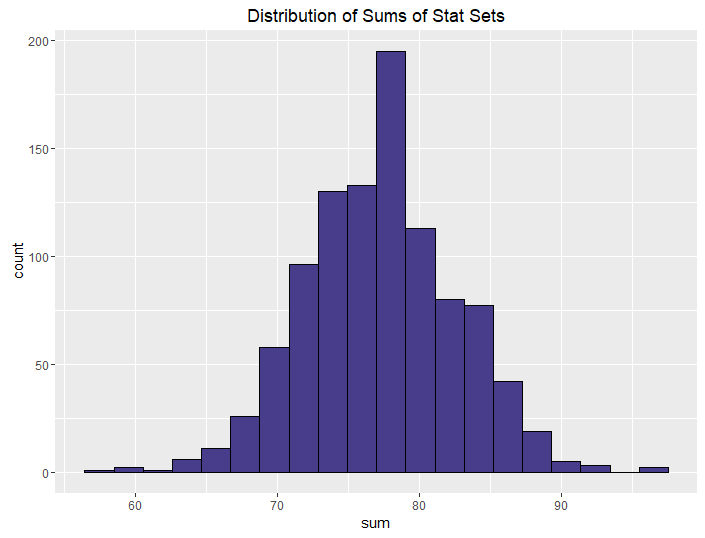
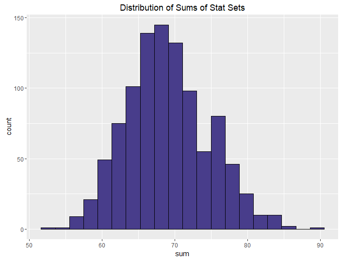
The above was repeated for each of the generated stat sets, resulting in the following distribution plots:

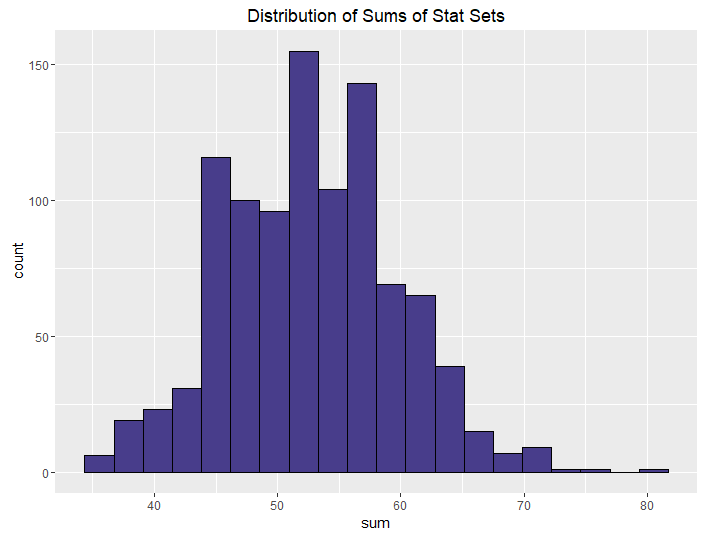
Roll 3, keep max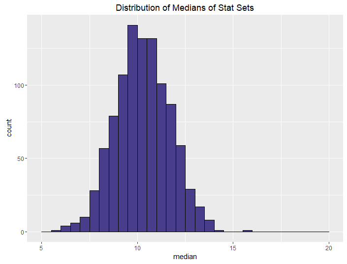
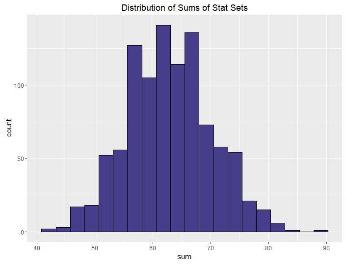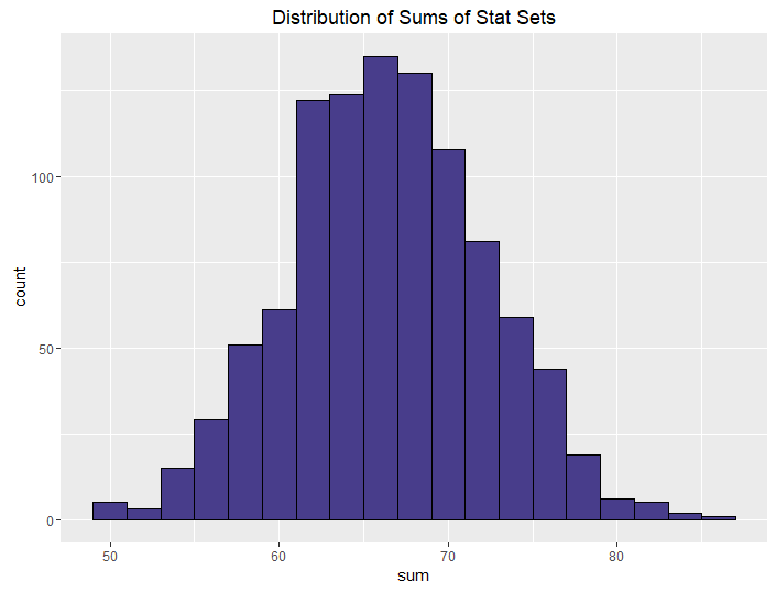
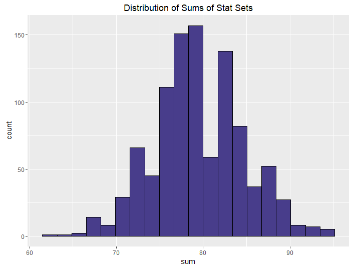
Roll 4, keep max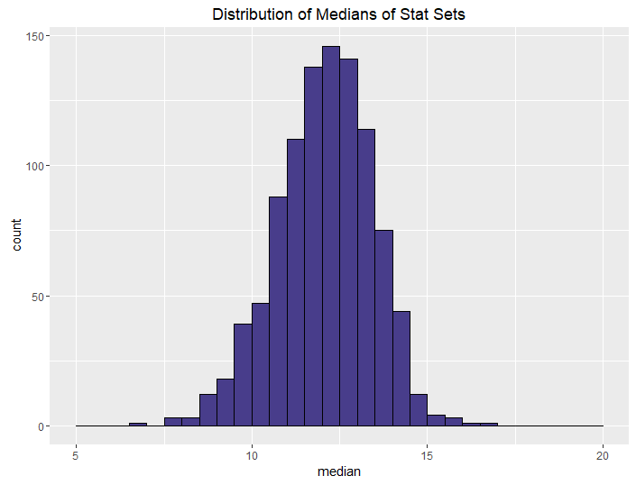
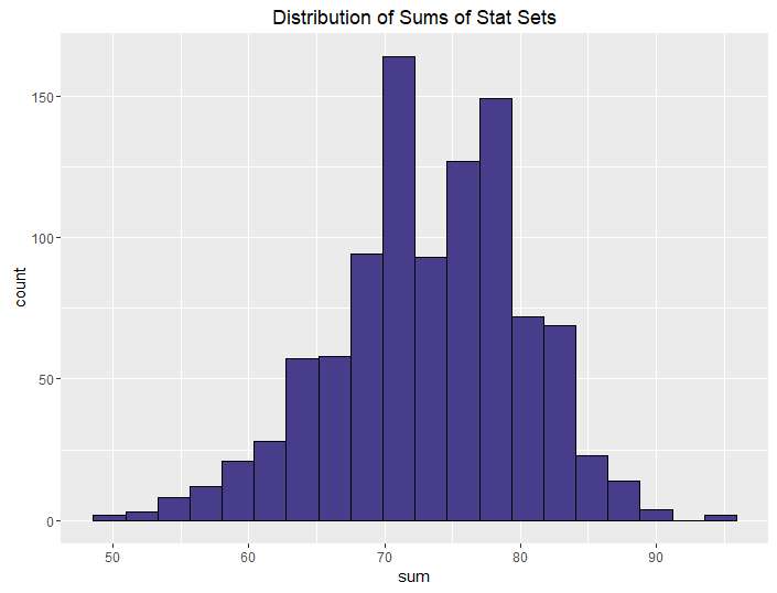Roll 4, keep min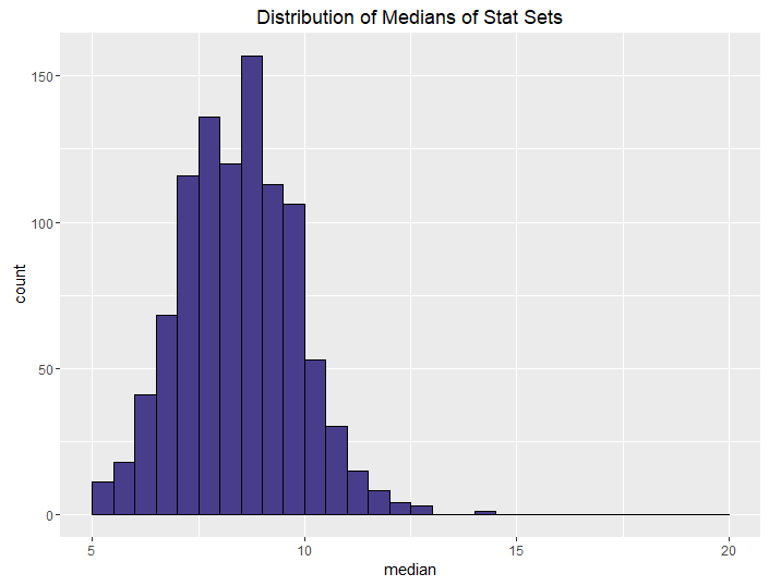
Best of 2, Roll 3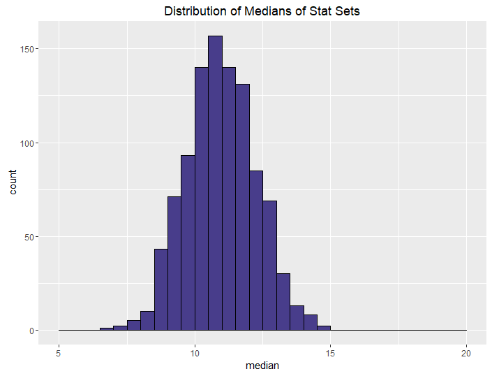
Best of 2, Roll 4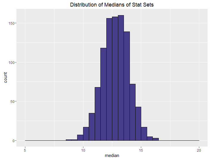
Best of 3, Roll 3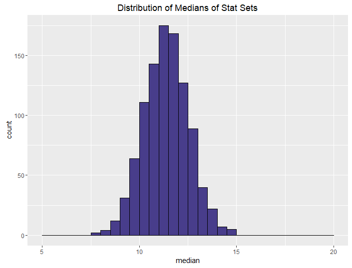
Best of 3, Roll 4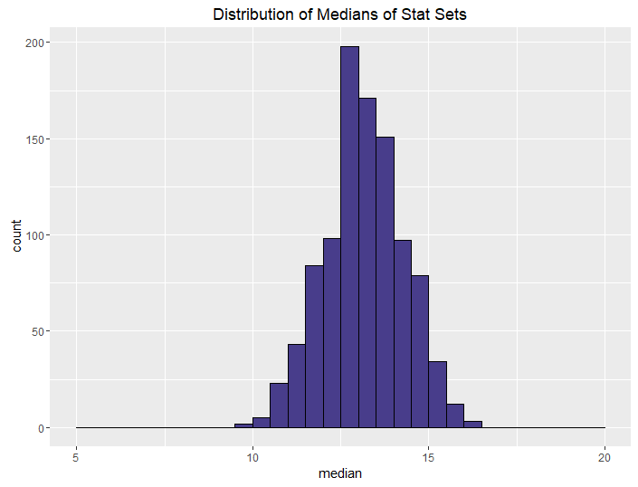
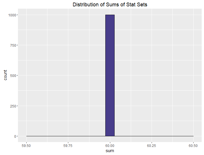
Inverse, Upper Bound (24, 22, 20)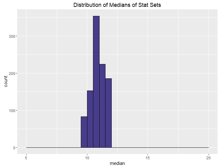
Inverse, Upper Bound (22, 20, 18)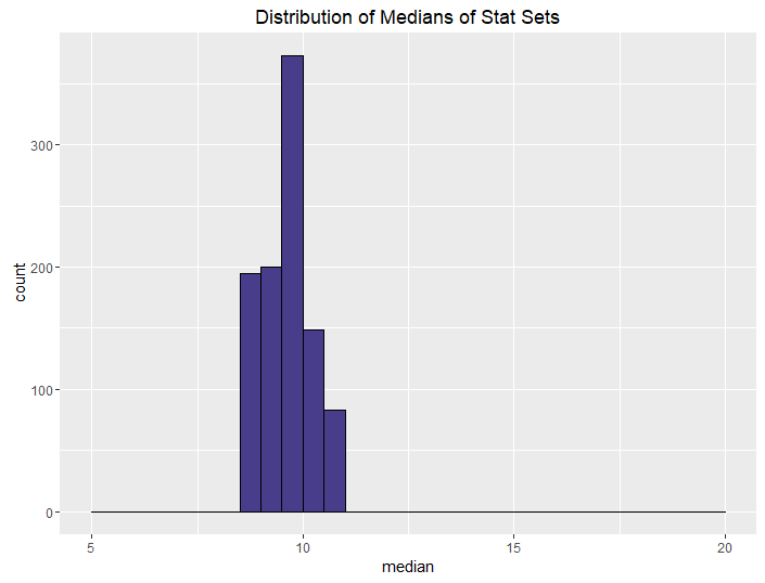

The conclusions from this aren’t all that surprising. The more rolls you use, the higher your median and sum are going to be, on average. What is neat, though, is how we can control the variance in stat sets by using different methods. This isn’t all that surprising either, but it is talked about less often when it comes to D&D stats.

The more opportunities you give your players to improve their stats when rolling, the better their stats are going to be, obviously. If you let your players roll 4 and drop 1 for each stat, they’re going to have better stats than if you let them roll 3. This is a choice you make as a DM: how powerful do I want my players to be? This differs from group to group and campaign to campaign.

What doesn’t vary is that we generally don’t want parties with massive discrepancies in power. When you have that in groups, it tends to breed a mixture of tension, nuisance, and boredom: the players with weak characters will alternately be bored and annoyed as their most powerful party member walks through challenges like they’re nothing as the rest of the party watches.

We can control this by using “best of” rolls. Note that the median and sums for the best of rolls don’t seem to change that much from their non-best-of counterparts. The median and sum are more determined by how many dice you roll (and subsequently drop) than by whether you generate one or two sets. If you want a powerful but balanced party, have your players do a best-of-2 rolling 4 dice. If you want an average but balanced party, do the same but only roll 3 dice. And if you want a weak but balanced party, have your players do a best-of-2 rolling 4 dice and keeping the minimum instead of the maximum.

At the far extreme of controlling variance is the “inverse” method. If you’re not a huge fan of randomness, you can use the inverse method to give your players the feeling of having rolled their dice without giving them the actual result of having done so. The inverse method controls the sum and median of your rolls. The DM need only set the upper bounds to determine exactly how strong they want their party to be.

Just to numerically demonstrate the point:

 1
 2
 3
 4
 5
 6
 7
 8
 9
10
11
12
13
14
15
16
17
18
19
20
21
22
23
24
25
26
27

# Variance in medians 
> var(stat_sets_3rm$median)
[1] 2.016391
> var(stat_sets_4rm$median)
[1] 1.868446
> var(stat_sets_bo2n3$median)
[1] 1.633033
> var(stat_sets_bo2n4$median)
[1] 1.348084
> var(stat_sets_bo3n3$median)
[1] 1.326064
> var(stat_sets_bo3n4$median)
[1] 1.265325

# Variance in sums 
> var(stat_sets_3rm$sum)
[1] 52.32621
> var(stat_sets_4rm$sum)
[1] 49.41758
> var(stat_sets_bo2n3$sum)
[1] 34.28188
> var(stat_sets_bo2n4$sum)
[1] 31.23015
> var(stat_sets_bo3n3$sum)
[1] 30.49885
> var(stat_sets_bo3n4$sum)
[1] 27.36714