Note: This post is still undergoing ‘renovation’ - images need to be cleaned up and mathematical notation inserted, but the core content is readable and correct.

Graphs are among the most basic and widely applicable mathematical structures. Modern applications in the study of social networks, spread of communicable diseases, computer networks, and many others, have made the study of graphs and their probabilistic counterpart, random graphs, especially relevant.

As a way of learning more about networks, I investigated algorithms for generating random graphs. Below, I have provided a basic introduction to the theory of random graphs, followed by implementations of a few random graph generating algorithms.

Mathematical notation is neglected here presently (due to a combination of learning how to format it in Hugo, and saving time).

Introduction to Random Graphs

A graph is defined as a pair of sets: one set of vertices, and another set of edges connecting those vertices. In undirected graphs, each edge can be represented as an unordered pair of vertices - whereas, in directed graphs, each edge must be an ordered pair.

A walk on a graph is a sequence of vertices and edges where each vertex in the sequence shares an edge with the next and the previous vertex. A path is a walk where no edges are repeated. Paths and walks can be open or closed: open if the starting vertex is different from the ending vertex, and closed otherwise.

Simple graphs are those which contain no self-loops and have at most on edge between each pair of vertices. A graph is connected if there exists a path from every vertex in the graph to every other vertex in the graph.

A random graph is defined as above, except that either the set of edges, the set of nodes, or both are generated probabilistically. There are many different models for generating random graphs, some of which will be discussed shortly.

Implementation of Graph Class

Before we can generate graphs, we need a graph class. This will make a few parts of the process easier - allowing us to abstract away some code that we don’t want to repeat.

 1
 2
 3
 4
 5
 6
 7
 8
 9
10
11
12
13
14
15
16
17
18
19
20
21
22
23
24
25
26
27
28

class Graph: 
	vertices = []
	edges = []
	def __init__(self, v, e):
		self.vertices = v 
		self.edges = e 
	def getAdjacentEdges(self, vertex):
		aedges = [e for e in self.edges if vertex in e]
		return(aedges)
	def getAdjacentVertices(self, vertex):
		aedges = self.getAdjacentEdges(vertex) 
		averts = set()
		for edge in aedges:
			for v in edge:
				if v != vertex:
					averts.add(v)
		return(list(averts))
	def DFS(graph, vertex):
		stack = []
		visited = set()
		stack.append(vertex)
		while stack:
			vert = stack.pop()
			if vert not in visited:
				visited.add(vert)
				for v in graph.getAdjacentVertices(vert):
					stack.append(v)
		return(list(visited))

Probably the only non-obvious part of the above class definition is the DFS method. This is a straightforward implementation of a Depth-First Search. Given a graph and a vertex, it explores every potential path away from that vertex to generate a list of all possible vertices that can be visited starting from that vertex. This will be useful later.

Random Graph Models, Part 1

The most simple and most famous model for generating and describing random graphs is the Erdos-Renyi model. The Erdos-Renyi (ER) model encapsulates at least two separate models which are, in the limit, equivalent.

The two models that the ER model may refer to are:

1. G(n, p): In this model, there exists a fixed number of nodes n and a fixed probability p of any two nodes being connected by a single, undirected edge. Random graphs in this model are generated by starting from a fixed set of vertices and connecting each pair with probability p. We call this the constructive model.

2. G(n, m): In this model, the number of nodes n and the number of edges m are both fixed, and the edges are randomly distributed among node parts. This model can be thought of as representing an ensemble of graphs obtained by sampling uniformly from all graphs with n vertices and m edges - giving it the name the sampling model.

For large n, these two models are equivalent. The intuition is simple: given G(n, p), we can construct a random variable m distributed as Bin(n(n-1)/2, p), yielding G(n, m).

Erdos and Renyi showed a number of interesting properties of graphs under this model, some of which we will examine later.

Implementing the Erdos-Renyi model

We first implement the constructive model for Erdos-Renyi random graphs. This model starts with n labeled vertices and a fixed probability p and subsequently generates edges. This part is relatively straightforward: given a list of vertices and a probability, we simply generate all possible combinations of size two, then we keep each edge with probability p.

1
2
3
4
5
6

def generateER_Graph(vertices, prob):
	possibleEdges = list(itertools.combinations(vertices, 2))
	edge_check = scipy.stats.bernoulli(prob).rvs(len(possibleEdges))
	realEdges = [possibleEdges[i] for i in range(0,len(edge_check)) if edge_check[i] == 1]
	er_graph = Graph(vertices, realEdges)
	return(er_graph)

Using this model, we generated a few graphs and display their vertex degree distributions as histograms below. MatPlotLib and NetworkX were used to display the graphs and generate the histograms below.

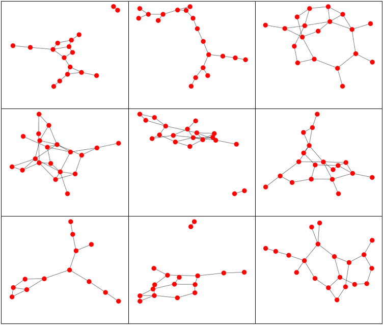
Erdos-Renyi Graphs generated with 20 vertices and p = 0.10. Note that if a vertex has no edges coming from it, it does not appear.

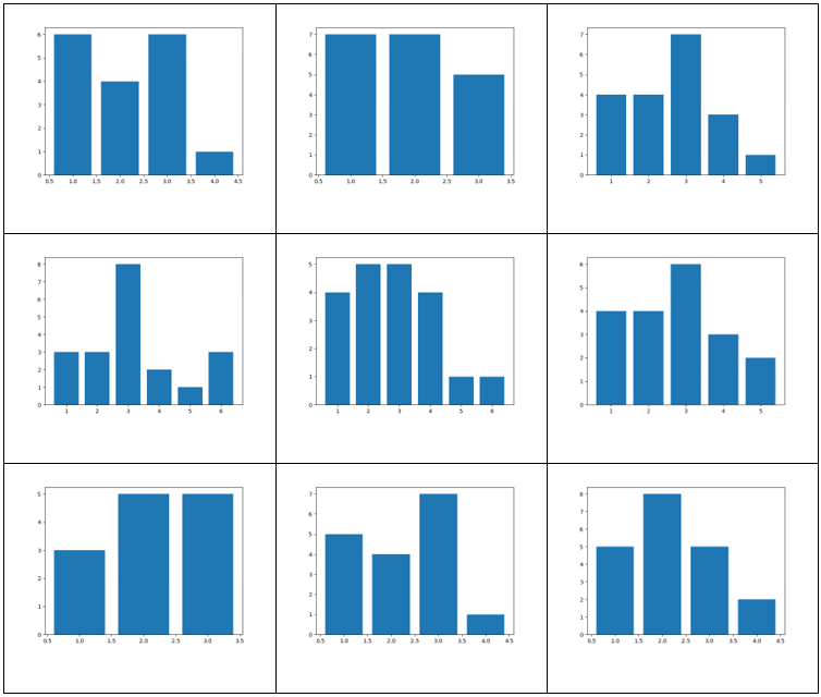
Histograms showing the vertex degree distributions corresponding to the graph in the same cell in the graph table.

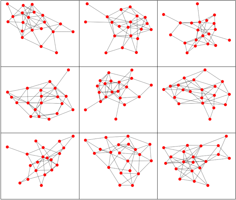
Erdos-Renyi Graphs generated with 20 vertices and p = 0.25. Note that if a vertex has no edges coming from it, it does not appear.

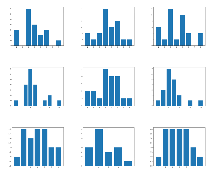
Histograms showing the vertex degree distributions corresponding to the graph in the same cell in the graph table.

This model allows us to demonstrate a result proven by Erdos and Renyi in their 1960 paper “On The Evolution of Random Graphs”. Erdos and Renyi showed that a critical transition occurs in random graphs as the number of edges approaches half the number of vertices in the graph. At this transition point, we see the emergence of a “giant component” - a connected component of the graph that outsizes all other components.

At this critical transition, the expected degree t of any one vertex in the graph passes from t < 1 to t > 1. Prior to this threshold, ER model graphs tend to be composed of many small components. Once this threshold is crossed, one giant component dominates the graph. This is reflective of the large degree of clustering that tends to be seen in real life networks.

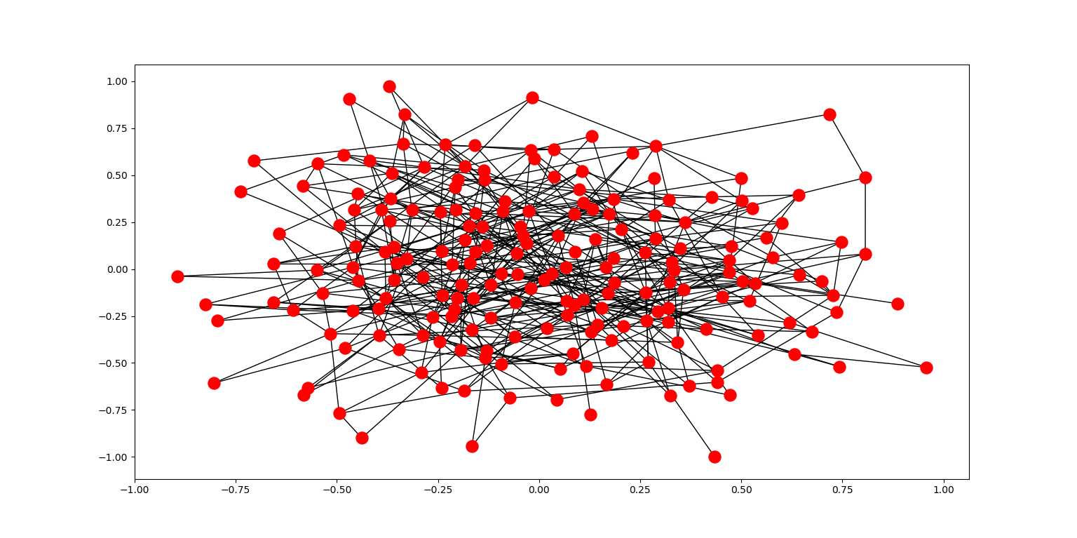
Below, an ER graph was generated using 200 vertices and a probability of 0.025 for any one potential edge to exist. The giant component in this graph should be fairly obvious:

Random Graph Models, Part 2

While its simplicity makes it possible to show a number of interesting results, it also limits the ER model’s applicability to real world networks. This is a result of the probability distribution defining its features: real world networks are rarely describable by treating every potential edge as independently having the same probability of existing.

We need a new model that allows graphs to be generated using arbitrary vertex probability distributions, and this exists in the form of the configuration model. The configuration model gives a simple algorithm for generating random graphs with a fixed number of nodes n , each of which has a number of edges connecting to it determined by an arbitrary probability distribution F. The algorithm follows:

1. Begin with n vertices and discrete pdf F
2. For each vertex, generate a single random value m from F
3. At each vertex, generate m "stubs"
4. Select two stubs at random and connect the two stubs to form an edge
5. Repeat the above step until all stubs are connected. 
6. If there are an odd number of stubs, simply remove the last remaining stub. 

This algorithm will often lead to graphs containing self-loops and multi-edges. If this happens and we don’t want graphs containing these, we simply throw out the graph, generate a new one, and repeat until we get a graph with no self-loops and multi-edges. We can also impose additional requirements, such as connectedness.

The downside of this model is that you can sometimes generate many graphs before arriving at a graph that meets your conditions. Unfortunately, simply removing multi-edges or self-loops when they occur or adding edges to connect an unconnected graph will cause the graph’s vertex distribution to no longer accurately reflect the chosen distribution.

Implementing the Configuration Model

The configuration model is implemented below. Here is where the depth-first search implemented in the original graph class is useful - using it, we can ensure that we only keep graphs that are connected. We also impose the additional requirements of no self-loops and no multi-edges. We use SciPy for its discrete probability distributions.

 1
 2
 3
 4
 5
 6
 7
 8
 9
10
11
12
13
14
15
16
17
18
19
20
21
22
23
24
25
26
27
28
29
30
31
32
33
34
35
36
37
38
39
40
41

def generateCM_Graph(degDist, vertices):
	# Function to generate test graphs that may or may not contain loops or multi-edges
	def genTestGraph(degDist, vertices):
		numVert = len(vertices)
		degrees = list(degDist.rvs(numVert))
		edges = list()
		dsum = sum(degrees)
		while(dsum > 0):
			v1 = random.randint(0, numVert-1)
			v2 = random.randint(0, numVert-1)
			if(degrees[v1] > 0 and degrees[v2] > 0):
				edges.append([vertices[v1], vertices[v2]])
				degrees[v1] = degrees[v1] - 1
				degrees[v2] = degrees[v2] - 1
				dsum = dsum - 2
		return(Graph(vertices, edges))
		
	# Uses above function to generate graphs, test them, and regenerate if needed
	goodGraph = False
	graph = genTestGraph(degDist, vertices)
	while(goodGraph == False):
		goodGraph = True
		# Checks that there are no self edges or multi-edges
		for i in graph.edges:
			count = 0
			if(len(i) != 2):
				goodGraph = False
				graph = genTestGraph(degDist, vertices)
				break 
			for j  in graph.edges: 
				if i[0] in j and i[1] in j:
					count = count + 1
			if(count > 1):
				goodGraph = False
				graph = genTestGraph(degDist, vertices)
		# Checks that all vertices are reachable 
		if(goodGraph == True):
			if not(collections.Counter(Graph.DFS(graph, graph.vertices[0])) == collections.Counter(graph.vertices)):
				goodGraph = False
				graph = genTestGraph(degDist, vertices)
	return(graph)

A few notes on this implementation. Note that there’s a nested function for generating graphs within the generateCM_Graph(.,.) function. This nested function does the heavy lifting of generating new graphs, while the rest of the function checks if this graph meets the conditions that we laid out for our configuration model. If the graph does not meet these conditions, yet another new graph is generated.

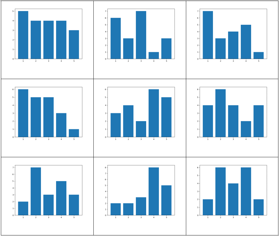
Graphs and associated vertex degree distributions can be found below.

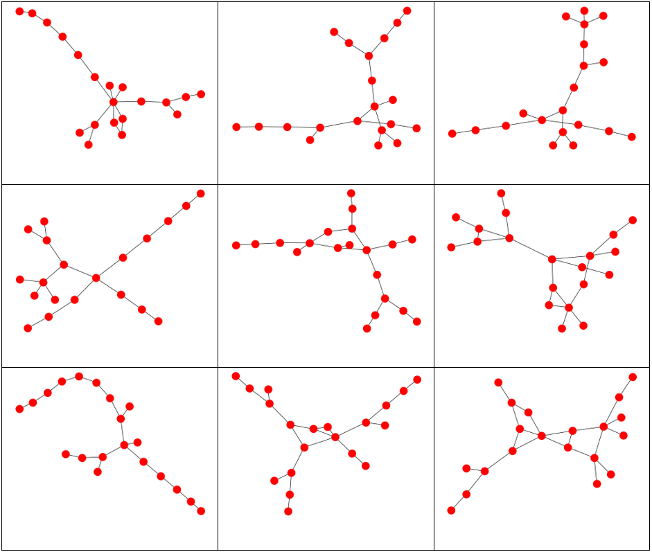
Here we generated graphs using an exponential distribution for the vertex distribution with a scaling parameter of 1. 20 vertices were used.

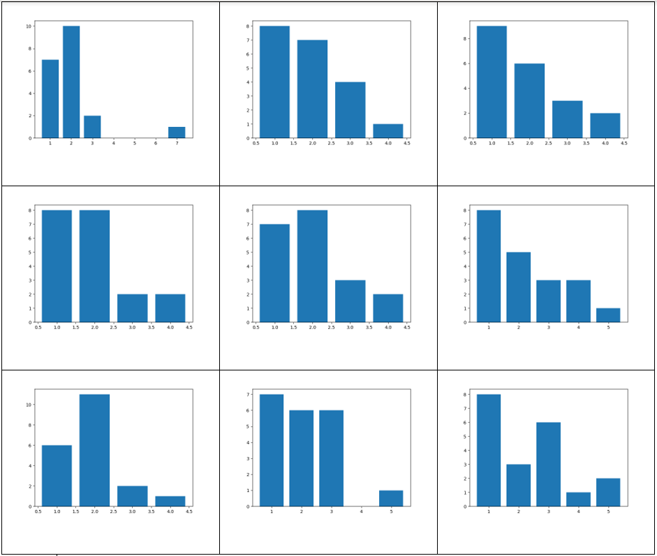
The vertex degree distribution histogram shows what we’d expect: most of the vertices have 1 or 2 degrees, reflecting the long “chains” seen in the above graphs.

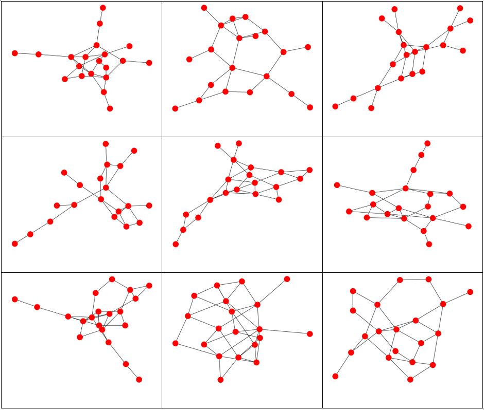
Here we generated graphs using a Uniform(1,5) distribution for the vertex distribution. 20 vertices were used. Note how much more interconnected the resulting graphs are than the exponential distribution graphs.

The vertex degree distribution histogram for the above graphs.